Reading notes on Causal-rCM: A Unified Teacher-Forcing and Self-Forcing Open Recipe for Autoregressive Diffusion Distillation (NVIDIA / Tsinghua, 2026). Organized as a concept-by-concept walkthrough, building from the ground up. Figures are self-contained SVGs (optimized for a light background).
The paper at a glance
The paper extends rCM — an advanced diffusion-distillation framework — to autoregressive (AR) video diffusion, the kind used for real-time streaming video and interactive world models.
The central idea is a forward/reverse complementarity carried over from rCM:
- Teacher-Forcing + Consistency Models (TF-CM) = the offline, forward-divergence, mode-covering component (stable; attends to clean ground-truth history).
- Self-Forcing + DMD (SF-DMD) = the on-policy, reverse-divergence, mode-seeking component (rolls out the student’s own generations; fixes exposure bias).
The recipe is a three-stage pipeline: (1) TF turns a bidirectional model into a causal/AR one; (2) TF-CM distills it into a few-step student; (3) SF-DMD refines on the student’s own rollouts.
Headline result: a distilled 2-step Wan2.1-1.3B model reaches VBench-T2V 84.63 at 1–2 sampling steps.
Part I — The paradigm
1. Autoregressive video diffusion & causal diffusion transformers
“Autoregressive video diffusion” is two ideas glued together on two different scales:
| Axis | Mechanism | Analogy |
|---|---|---|
| Across time (frames/chunks) | Autoregressive: generate block i conditioned only on past blocks — $p_\theta(x_0)=\prod_{i} p_\theta(x_0^i \mid x_0^{<i})$ | an LLM writing token by token |
| Within a block (one frame/chunk) | Diffusion: denoise that block from noise to clean | a normal image diffusion model |
One-liner: autoregressive across frames/chunks, diffusion denoising within each frame/chunk.
A causal diffusion transformer = a Diffusion Transformer (DiT) backbone whose temporal attention is masked so each frame attends only to the past (the GPT-style causal mask). That causal mask is what makes streaming, KV caching, and interactivity possible.
There is another major paradigm
| Bidirectional video diffusion (the original default) | Autoregressive video diffusion (this paper) | |
|---|---|---|
| Attention over time | Full — every frame sees every other | Causal — each frame sees only the past |
| How it generates | Denoise all frames jointly in one shot | Generate frame/chunk by chunk |
| Latency | High — must finish the whole clip | Low — stream as you go |
| Length | Fixed at train time | Open-ended / infinite |
| Interactive? | No | Yes (inject actions mid-stream) |
| KV caching | No | Yes (like LLMs) |
| Examples | Sora-style, base Wan2.1, HunyuanVideo | Self-Forcing, CausalForcing, Causal-rCM |
It’s the same DiT — only the attention mask changes
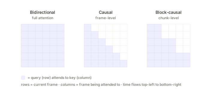 Rows = the query frame; columns = the key frame. Filled = attention allowed. Bidirectional fills everything; causal keeps the lower triangle; block-causal is full within a chunk but causal across chunks.
| Pattern | A frame can see… | Used by | Buys you |
|---|---|---|---|
| Full / bidirectional | all frames (past + future) | joint video diffusion | max coherence; no streaming/caching |
| Causal (frame-level) | only strictly past frames | frame-wise AR (c1-1) |
lowest latency, finest interactivity |
| Block-causal (chunk-level) | past chunks + own chunk, fully | chunk-wise AR (c3-3) |
richer intra-chunk motion + streamable |
Note: the spatial axis is always full/bidirectional. Only the temporal axis gets masked. Cosmos 3 states this explicitly — within one frame, all spatial tokens attend freely.
2. What the AR design unlocks: streaming, interactivity, KV caching
The single insight behind all three: the causal factorization makes the past immutable. Once a frame is generated, it never changes — and every capability follows from that.
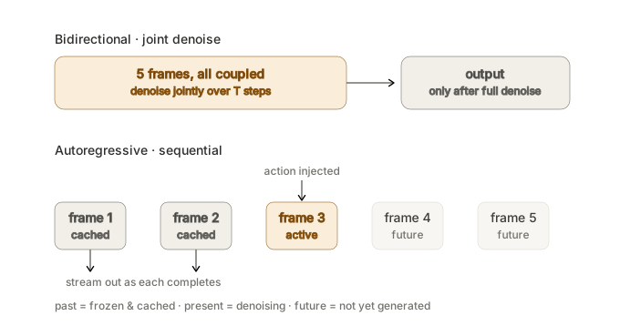 Bidirectional denoises all frames together and outputs only at the end. Autoregressive finalizes frames one at a time: the past is cached and streamed out, the present denoises, an action can be injected, and the future isn’t generated yet.
- Streaming — a finished frame is final (the causal mask forbids the past from depending on the future), so you can emit it immediately while later frames still compute. In bidirectional joint denoising, frame 1’s pixels depend on frame 50 throughout the shared denoising process — nothing is “done” until the very last step.
- KV caching — a frozen past frame has frozen key/value vectors → compute once, reuse forever. In bidirectional, every frame’s K/V changes at every denoising step, so there’s nothing stable to cache.
- Interactivity / world models — sequential generation creates a seam between frame i and i+1 where you can inject an action $A_i$, turning the model into a transition function $(V_i, A_i) \to V_{i+1}$ — a simulator. Bidirectional has no seam.
Why you need both ingredients
| You have… | …but you’re missing | Result |
|---|---|---|
| Diffusion only (bidirectional) | the causal factorization | gorgeous frames, but a frozen offline clip |
| Autoregression only (plain regressor) | diffusion within each frame | streamable, but blurry frames |
| Both fused = AR video diffusion | — | sharp, diverse frames and streamable/steerable |
Mental model: AR video diffusion = the LLM generation machinery, with the “token” upgraded from a word to a whole frame painted by diffusion. The AR half supplies system properties; the diffusion half supplies visual quality.
3. Spatial vs. temporal axes — and why different masking
After VAE compression, a video is a 3-D block of tokens: time × height × width. Each token’s identity is (which frame, where in the frame).
- Spatial axis = where inside one frame a token sits (the H×W patch grid).
- Temporal axis = which frame the token belongs to.
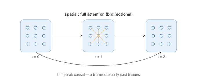 Within one frame, every patch attends to every other (full). Across frames, attention only flows forward in time (causal).
The reason for the asymmetry: causality is a property of time, not space.
- Within a frame, nothing is “before” or “after” — every patch must negotiate with every other to render a coherent image. Masking would be harmful. So spatial attention is full.
- Across frames, there is a direction. To get streaming/caching/interactivity, a frame may only depend on earlier frames. So temporal attention is causal.
Comic-strip analogy: inside each panel the artist composes everything together (spatial = full); the panels are drawn in story order, each continuing the last (temporal = causal).
Part II — Why diffusion at all
4. The denoiser, n-step denoising, and the blurry-mean problem
Why a denoiser inside each frame? Because generating one frame is itself a hard generative problem. Given the context, there are many plausible next frames — the distribution $p(\text{frame}\mid\text{context})$ is multimodal. A denoiser lets you draw one sharp sample instead of collapsing the distribution.
What “n-step denoising” means. A diffusion model walks a chain of decreasing noise levels, calling the denoiser once per step:
\[z \;(\text{noise}) \to \tilde{x}_{t_{N-1}} \to \dots \to \tilde{x}_{t_1} \to \tilde{x}_0 \;(\text{clean})\]Each arrow = one network evaluation (NFE). A pretrained model needs ~50 steps; distillation compresses that into 1–4. The paper even varies N per chunk (the first chunk is hardest and gets more steps):
| Variant | First chunk | Later chunks |
|---|---|---|
| 4-step | 4 | 4 |
| 2-step | 4 | 2 |
| 1-step | 4 | 1 |
(One subtlety: clean-context AR costs N + 1 NFEs per chunk because of an extra cache-encoding pass; the “noisy context” trick drops the +1.)
Why a deterministic regressor blurs. Train a network $f$ with MSE and the optimal solution is the conditional mean $\mathbb{E}[\text{frame}\mid\text{context}]$. The mean of a multimodal distribution sits in the empty valley between the modes — an average of sharp-but-different images, which cancels high-frequency detail into mush.
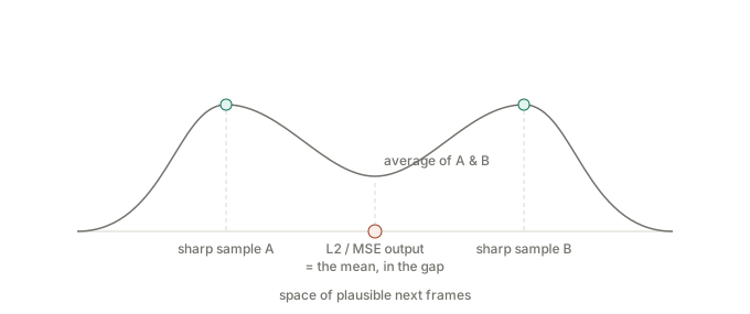 The two peaks are valid sharp samples. The L2-optimal output is their average, which falls in the low-probability gap → blur, and zero diversity.
How diffusion escapes it (even though it also uses an MSE-style loss):
- Its prediction is conditioned on a noisy version of the target $x_t$ — at low noise the target already contains most of the detail, so the model only predicts a tiny near-deterministic residual. The averaging happens over a tiny gap, never the whole image.
- The random seed selects which mode you land in. Different seeds → different sharp samples.
5. VAE, latent space, and latent tokens
Running diffusion on raw pixels is hopelessly expensive, so modern models do latent diffusion: a VAE (Variational Autoencoder) compresses pixels to a small code, all diffusion happens in that code space, and the decoder renders pixels at the end.
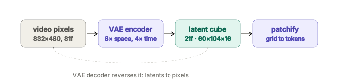
- Latent = a learned, compressed, abstract representation (not the raw observable thing). Latent space = the vector space those codes live in.
- Latent tokens = the VAE-compressed cube, chopped into patches; each patch is one token living in VAE latent space.
- Latent space in LLMs = the model’s internal hidden representations (embeddings → evolving hidden activations). No VAE, but the same core idea: meaning encoded geometrically in a learned vector space.
Worked example of the spatial axis (the paper’s setup): a 832×480 frame → ~104×60 latent positions (≈8× spatial compression), each a 16-dim vector; 81 frames → 21 latent frames (4× temporal). Patchify (e.g., 2×2) → a few thousand spatial tokens per frame. One spatial token = “the patch at row 30, column 50 of latent frame 7.”
6. Vision supertokens (Cosmos 3)
A “vision supertoken” bundles all spatial tokens of one frame into a single unit. The benefit is a clean decoupling of the two axes:
- Simple causal rule — instead of per-patch bookkeeping, the rule is just “supertoken i can’t see supertoken j > i,” while everything inside a supertoken stays fully bidirectional.
- Clean action alignment — one supertoken = one timestep = one decision point, so action $A_i$ cleanly controls the $V_i \to V_{i+1}$ transition (a null action is inserted before $V_0$).
- Natural caching unit — a whole frame’s K/V is committed/read at once.
7. Diffusion as a process; multimodality and seeds
“Diffusion” = two processes, not just denoising:
- a forward (noising) process — fixed, not learned — that adds Gaussian noise until data becomes pure noise;
- a reverse (denoising) process — learned — that undoes it.
Generation = run the reverse process from noise to data.
Is the distribution really multimodal? Yes, with direct evidence: (a) different seeds on the same prompt yield genuinely different valid outputs; (b) MSE next-frame predictors empirically blur — the fingerprint of multimodality; (c) given a prompt + a few frames, enormous detail is underdetermined (high entropy).
Seeds and modes — the correct picture (a common misconception to avoid):
One generation draws one seed → it flows to one mode → one sharp sample. Modes are never fused. Diversity comes from re-running with a different seed.
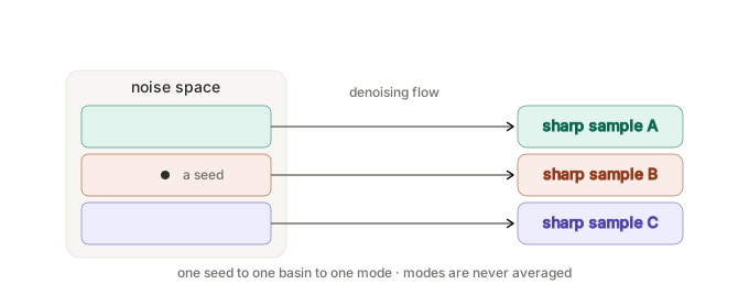 The deterministic ODE sampler partitions noise space into basins (like a watershed). Your seed = where the raindrop lands → which basin → which single mode.
Averaging modes is the bad thing (the MSE regressor → blur). Diffusion does the opposite: it commits to one mode per seed → sharp. “Commit, don’t average.”
Part III — Representations & objectives
8. LLM embeddings & hidden activations
Why a high-dimensional vector? A word is a discrete symbol; a network computes with continuous vectors, so you must embed it. High-dimensional because meaning is many-faceted — each dimension can encode a different attribute (animacy, size, tense, sentiment…), letting all of a word’s relationships hold at once. The famous king − man + woman ≈ queen only works with enough dimensions.
Why the evolving hidden activations are “meaning.” The embedding is context-free (“bank” is identical everywhere). As the vector passes through layers, attention mixes in context, rewriting it to reflect meaning-in-context. A hidden activation is literally a float vector (e.g., length-4096); one per token per layer.
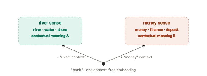 Same input symbol, two different hidden activations after the attention layers. That drift is the model representing meaning.
9. Distillation, and the teacher trajectory as ground truth
Distillation = transfer a slow, high-quality teacher’s skill into a fast student. The teacher needs ~50 steps; the student should match it in 1–4. The student learns this from the teacher, not from raw data.
The teacher is a pretrained diffusion model. For any noisy point $x_t$ it defines a deterministic path (its PF-ODE) down to a clean $x_0$ — this path is the ground-truth reference (it’s computable by running the teacher). The consistency property: every point on one path shares the same endpoint $x_0$, so the student can leap from any noise level straight to it (“one big jump = many small steps”). CM enforces this locally (between adjacent timesteps), and local consistency chains into the global endpoint; sCM uses the instantaneous tangent (the JVP).
10. Two orthogonal axes: TF/SF vs. CM/DMD
A crucial untangling. These are independent axes, not synonyms:
- Loss (what you optimize): CM (consistency, trajectory-matching, forward divergence) vs DMD (distribution-matching, reverse divergence).
- Context (what history the model conditions on): Teacher-Forcing (clean ground-truth past) vs Self-Forcing (the model’s own rollout, on-policy).
So teacher-forcing is not CM, and self-forcing is not DMD — the paper simply pairs them on the diagonal.
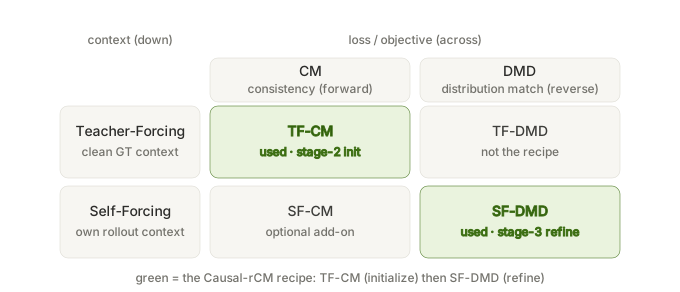
Why the diagonal pairing:
- TF pairs with CM — clean, stable, offline context is exactly where trajectory-matching (mode-covering) works → a stable initialization.
- SF pairs with DMD — the model’s own imperfect rollouts are the real inference distribution; matching distributions there (mode-seeking) directly fixes exposure bias → on-policy refinement.
The whole bet: TF-CM to initialize, then SF-DMD to refine, mirroring rCM’s “forward for coverage, reverse for quality” philosophy.
11. ODE and the PF-ODE
An ODE (Ordinary Differential Equation) is $\frac{dx}{dt} = f(x,t)$: it gives the velocity at every point, not the path. To get the path, you integrate (follow the velocities from an initial point). “Ordinary” = derivatives in one variable (time).
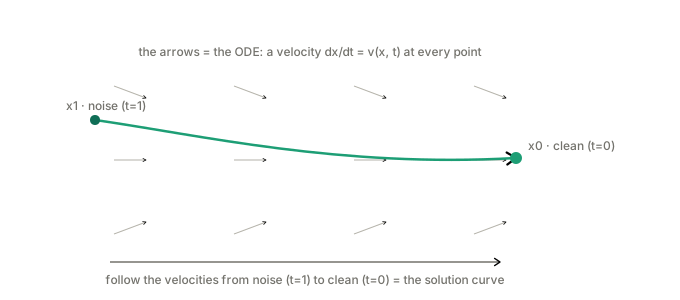 The arrows are the rule; the curve is the solution. Mapped onto diffusion: start at noise (t=1) and follow the field to clean (t=0).
In the paper, PF-ODE (probability-flow ODE) is exactly this:
- the teacher is the velocity field $v_{\text{teacher}}(x_t,t)$;
- generation = solving the ODE from noise down to a clean frame (the “teacher trajectory”);
- n-step denoising = solving it numerically (Euler etc.); more steps = better integration;
- “probability flow” = the deterministic twin of the stochastic diffusion (same marginals) — which is why one seed → one deterministic trajectory → one mode;
- CM/sCM live on this curve (same endpoint; the tangent is the JVP).
Part IV — rCM & training configuration
12. rCM in depth
rCM = score-regularized continuous-time consistency model (Zheng et al., Oct 2025; the bidirectional predecessor of this paper).
- Problem it fixes: pure continuous-time consistency (sCM) underperforms at large scale on fine detail, due to error accumulation and the mode-covering nature of its forward-divergence objective (spread-out densities, soft detail).
- The fix: add score distillation (DMD-style) as a “long-skip regularizer” — a mode-seeking reverse-divergence term that sharpens quality while keeping diversity. The two are complementary (forward = coverage, reverse = quality). This is the forward/reverse complementarity in its original form.
- Enabling infrastructure: a parallelism-compatible FlashAttention-2 JVP kernel (so the continuous-time tangent can be computed through fused attention on 10B+ param video models), plus stable time-derivative computation. Causal-rCM inherits this kernel and adds custom masks.
- Training style: a single joint stage — no GAN tuning, no multi-stage pipeline, minimal hyperparameter search.
- Results: 1–4 steps, ~15–50× speedup, matching DMD2 on quality while keeping better diversity.
vs. Causal-rCM: rCM is bidirectional and trains CM+DMD jointly. Causal-rCM lifts the same philosophy to the autoregressive setting, pairs the objectives with causal contexts (TF-CM, SF-DMD), and runs them sequentially in stages (joint training lowers the ceiling in the causal case).
13. Table 3 training parameters, decoded
Fake-score optimizer. DMD needs the student’s own (intractable) score, so it trains an auxiliary fake-score network $\varphi$ on student samples to estimate it — a “critic” with its own AdamW optimizer. Only appears in Stage 3 (SF-DMD).
CFG scale (classifier-free guidance). A knob for how hard to obey the prompt: $\text{pred} = \text{uncond} + \text{scale}\times(\text{cond}-\text{uncond})$. Higher = stronger prompt adherence, punchier contrast, less diversity. CFG 5.0 generates the teacher’s training data; CFG 3.0/5.0 are used when querying the teacher during distillation. The student bakes guidance into its weights → no CFG needed at inference (part of the speedup).
Euler sampling + shift. Euler is the simplest first-order ODE solver; “100-step Euler” is how the teacher solves its PF-ODE to make training data. Shift reparameterizes where the steps land, via $t’ = \frac{s\,t}{1+(s-1)t}$:
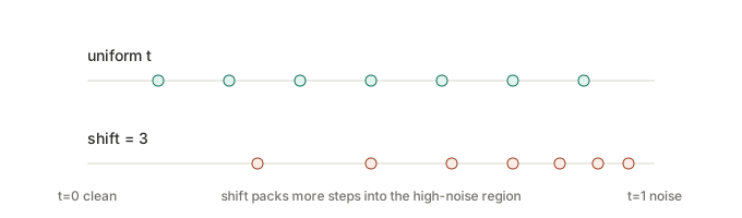 A shift of 3 packs more steps into the noisy end, where high-resolution video needs the most care.
RF sampling schedules. RF = Rectified Flow ($\alpha_t = 1-t,\ \sigma_t = t$, so t=1 is noise, t=0 is clean). An “RF schedule” is the explicit list of timesteps the few-step sampler stops at — e.g. the 4-step sampler uses $[15/16, 5/6, 5/8]$.
TF / DF time-sampling + weighting rows:
- $p_G = \text{UniformShift}(5)$ — draw the training noise level $t$ uniformly on $[0,1]$, then apply a shift of 5 (biasing toward the noisy regime).
- shared $t$ (TF) vs random per-chunk $t$ (DF) — TF applies one shared noise level across the clip while attending to clean history; DF gives each chunk its own independent noise level (its defining feature, improving robustness to imperfect context).
- Gaussian-bell weight (TF) vs no weight (DF) — TF emphasizes mid-range noise levels with a bell-shaped loss weight; DF uses flat weighting.
Mini-glossary
| Term | One-line meaning |
|---|---|
| AR video diffusion | Autoregressive across frames, diffusion within each frame |
| DiT | Diffusion Transformer (transformer as the denoiser) |
| TF / SF | Teacher-Forcing (clean context) / Self-Forcing (own rollout) — a context choice |
| CM / dCM / sCM | Consistency Model / discrete-time / continuous-time — a loss (forward divergence) |
| DMD | Distribution Matching Distillation — a loss (reverse divergence) |
| VAE | Variational Autoencoder; compresses pixels ↔ latents |
| latent token | A patch of the VAE-compressed video, in latent space |
| (PF-)ODE | Probability-flow ODE; the deterministic noise→data velocity field |
| JVP | Jacobian-vector product; the instantaneous tangent sCM needs |
| NFE | Number of Function Evaluations (≈ denoising steps) |
| CFG | Classifier-free guidance; prompt-adherence knob |
| RF | Rectified Flow noise schedule |
| rCM | Score-regularized continuous-time CM (CM + DMD, jointly) |
| exposure bias | Train/test gap: at inference the model conditions on its own imperfect history |